

Startup Loss The Overlooked Waste with a Massive Impact on OEE
Often dismissed as a “normal” part of production, this waste can actually be measured, analyzed, and minimized. By leveraging Cycle Time data, manufacturers can systematically unlock higher efficiency. Solwer breaks down the root causes of Startup Loss, delivers actionable solutions, and demonstrates how to master Cycle Time Analysis to eliminate this hidden waste.
What is Startup Loss?
You May Also Like


Startup Loss refers to the inefficiencies and waste incurred during the “start of production.” This typically occurs when firing up machines for the day or immediately following a shift change.
In the LABD framework, “Model Change” is strictly categorized separately from Startup Loss. However, there is one exception: if a model change occurs exactly at the start of a shift, the entire duration is classified as Startup Loss.
During this initial phase, the equipment is not yet optimized. Machines may require parameter tuning, temperatures might not be fully stabilized, operating speeds can fluctuate, and control systems may not yet be running at peak performance. Simultaneously, operators are still in the preparation phase—verifying raw materials, configuring tooling, or conducting the First Piece Trial.
This combination of machine warm-up and human preparation results in highly visible losses, including:
- Setup and Adjustment Delays: Time spent waiting for machines to be calibrated and ready.
- Ad-hoc Troubleshooting: Unplanned stoppages to resolve immediate, unforeseen issues on the line.
- Repeated Trial Runs: Multiple test cycles are required before meeting the quality baseline.
- Initial Scrap (Defects): Yield loss generated during the first production lot.
- Sub-standard Cycle Times: Production is running at reduced speeds before reaching the standard cycle time.
While these activities are often accepted as “routine steps” of starting a shift, from an engineering and efficiency standpoint, they are absolute losses. Because they do not yet generate true Value Added to the final product, they directly erode your overall productivity.

16 Where Do the 16 TPM Losses Fit in the Production System?
In the framework of Lean Manufacturing and OEE (Overall Equipment Effectiveness) evaluation, critical production wastes are categorized into six distinct types, known as the Six Big Losses. These are the primary factors that directly degrade machine efficiency and overall production capacity.
The Six Big Losses concept is engineered to help manufacturing facilities “visualize hidden losses” and analyze them systematically. To provide actionable data, these losses are structured into three major groups that perfectly align with the three core pillars of OEE: Availability, Performance, and Quality.
1. Availability Loss
This category encompasses losses that force the machine to “stop” or prevent it from operating during scheduled production hours.
1.Breakdown Loss (Equipment Failure)
- Unplanned Stoppages: Production halts due to equipment failure or malfunctions.
- Maintenance Downtime: Requires reactive repair and maintenance time.
- Capacity Drain: Directly eliminates available production capacity.
2. Setup & Adjustment Loss (Configuration & Tuning)
- Changeover Time: The duration required to switch from one product model to another.
- Calibration: Time spent adjusting and configuring machine settings prior to production.
- Trial Runs: Includes test production cycles before transitioning to standard operation.
This is the first critical point connected to Startup Loss, as the startup phase typically occurs immediately following a setup or changeover.
2.Performance Loss
This occurs when the machine is technically running, but operating “slower than the optimal standard.”
Minor Stops (Frequent, Brief Interruptions)
- Micro-Stoppages: Minor equipment jams or brief interruptions.
- Quick Interventions: Requires quick, minor adjustments or fixes by the operator.
- High Frequency: The downtime is not severe enough to be classified as a Breakdown, but it occurs frequently enough to disrupt continuous flow.
Reduced Speed Loss (Operating Below Standard Speed)
- Sub-Optimal Cycle Time: The equipment runs slower than its stated Ideal Cycle Time.
- Quality Precautions: Operators intentionally reduce machine speed to mitigate potential quality defects.
- Initial Instability: The system has not yet reached a stable, steady state during the early phase of production.
During the Startup phase, machines typically cannot yet operate at full speed or peak efficiency, which directly contributes to this Reduced Speed Loss
3.Quality Loss
This category represents the losses incurred when producing units that “fail to meet quality standards.”
Production Defects (Steady-State Rejects)
- In-Process Defects: Defective parts or scrap generated during normal, continuous production.
- Scrap or Rework: Non-conforming units that must be repaired, reprocessed, or discarded entirely.
Reduced Yield / Startup Defects (Initial Phase Yield Loss)
- Startup Scrap: Defects produced immediately after firing up the machine.
- Lot Instability: Unstable output and variations during the first production run.
- Unoptimized Quality: Production occurs before machine parameters are fully stabilized.
- Tuning Requirements: Requires further adjustment and calibration before consistently meeting standard quality baselines.
Startup Loss falls directly under this specific category. It is the tangible waste generated during the initial production phase before the manufacturing process achieves a reliable, Stable Condition.
Where Does Startup Loss Fit in the Six Big Losses?
Startup Loss is not a standalone, isolated metric. Instead, it is “embedded across multiple categories,” specifically impacting the following:
- Reduced Yield / Startup Defects: Its primary location, accounting for the scrap and defective parts generated during the initial run.
- Setup & Adjustment Loss: Driven by the fact that the startup phase immediately follows machine setup and changeovers.
- Reduced Speed Loss: A result of machines intentionally or inherently running below peak cycle times during the warm-up period.
Ultimately, Startup Loss acts as the “intersection” of multiple inefficiencies. While often dismissed by operators as a normal routine, it is fundamentally a systemic loss that continually drains overall plant efficiency.
How Does Startup Loss Impact OEE?
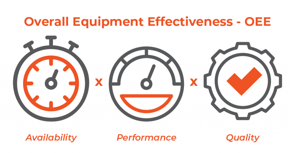
OEE (Overall Equipment Effectiveness) is the fundamental metric for measuring the overall efficiency of your equipment and manufacturing processes. It is calculated using three core components:
OEE = Availability × Performance × Quality
While many organizations fixate on unexpected breakdowns or steady-state defects, in reality, Startup Loss silently and simultaneously degrades all three OEE components—often with a much more severe impact than anticipated.
Want to dive deeper into mastering these metrics? Download Solwer’s full-version OEE e-book today!
1. Impact on Availability
Availability = Operating Time / Planned Production Time
During the Startup phase, several delays typically occur:
- Adjustment Time: Time spent tuning and calibrating equipment settings.
- Trial Production: Running test cycles prior to Quality Control (QC) approval.
- Ad-hoc Troubleshooting: Halting the line to resolve unforeseen technical hiccups.
- Idle Waiting: Delays caused by waiting for raw materials or first-lot quality validation.
Even if the machine is physically “powered on,” if it is not producing standard-quality parts, it is not generating true output. This leads to:
- Wasted Capacity: Planned Production Time is consumed without yielding saleable products.
- Direct Availability Drop: An immediate, negative impact on your Availability metric.
Solwer Insight: If your plant accepts a 30-minute startup delay every day, you are instantly bleeding 15 hours of lost production capacity every single month.
2.Impact on Performance
Performance = Actual Operating Speed / Ideal Cycle Time
The Startup phase is typically characterized by the following conditions:
- Sub-Standard Speeds: Machines operating significantly slower than the Standard Cycle Time.
- Manual Speed Throttling: Operators intentionally reducing line speeds as a precaution to monitor and control initial quality.
- System Instability: Equipment not yet reaching optimal operating temperatures or steady-state conditions.
Even in the absence of absolute downtime, operating below the optimal speed leads to:
- Performance Ratio Drop: A direct and immediate decline in your Performance metric.
- Sub-Optimal Throughput: Units produced per hour falling well below the machine’s true capability.
- Hidden Capacity Drain: A silent, unnoticed reduction in your overall daily production volume.
Solwer Insight: If your standard Cycle Time is 30 seconds per part, but your startup phase runs at 45 seconds per part, you are effectively bleeding 50% of your production potential during that entire window.
3. Impact on Quality
Quality = Good Parts / Total Parts Produced
Startup Loss strikes hardest in this specific metric due to:
- First-Lot Defects: The inevitable generation of scrap during the initial production run.
- Scrap and Rework: Non-conforming units that immediately require reprocessing or disposal.
- Unstable Parameters: Machine settings fluctuating before reaching optimal, steady-state temperatures or pressures.
- Unsettled Processes: The overall manufacturing process not yet being fully locked in.
Defects generated during this crucial startup window lead to:
- Plummeting Quality Rate: A direct, negative hit to your overall Quality score.
- Inflated Unit Costs: Higher cost per good part due to wasted operational time.
- Zero-Revenue Waste: Consuming valuable raw materials and energy without generating any saleable product.
Solwer Insight: In many manufacturing facilities, startup scrap alone accounts for a staggering 20–40% of the total daily defects.

Why is Startup Loss Often Overlooked?
Often dismissed as an “unavoidable cost of doing business,” Startup Loss is a dangerous blind spot. Because it happens daily—during morning start-ups or routine changeovers—it becomes ingrained in the workflow. Without dedicated KPIs or real-time data tracking, this routine inefficiency goes completely unchecked.
However, aggregating these daily delays reveals weeks of lost capacity annually. This systemic negligence directly causes:
- Inflated Unit Costs: Wasted time, energy, and materials drive up expenses.
- Diminished Capacity: A severe drop in overall throughput and potential output.
- Delayed Deliveries: Unnecessary bottlenecks that disrupt your supply chain.
- First-Lot Defects: Avoidable scrap and rework right out of the gate.
Operator Burnout: Unnecessary manual adjustments and shop-floor stress.
Why is Startup Loss More Dangerous to OEE Than You Think?
While Startup Loss might seem like a brief, harmless delay before production begins, its impact on OEE is profoundly destructive. It is not a single, isolated event—it is a cumulative, systemic leak hidden within your top-line metrics.
1. A Daily Drain: The Compounding Effect (Cumulative Loss)
Startups do not just happen when the factory opens. They strike repeatedly throughout your operations:
- Shift Changes: Initiating a new shift.
- Changeovers: Transitioning between product models.
- Post-Maintenance: Firing up machines after repairs.
- Intraday Stoppages: Restarting the line after unexpected downtime.
Losing 20–30 minutes a day might look acceptable on a daily shift report, but the aggregate math tells a different story:
- 30 mins/day × 26 days = 13 hours/month
- 13 hours/month × 12 months = 156 hours/year
That is nearly an entire month of production capacity wiped out—and most facilities do not even track it. The true danger of Startup Loss is not in the individual delay, but in its relentless frequency and compounding damage to your bottom line.
Many facilities calculate OEE as a daily aggregate, failing to isolate the startup phase from steady-state production. This creates a dangerous illusion:
- Averaged-Out Metrics: High performance during the rest of the shift overcompensates for the disastrous startup window.
- Buried Bottlenecks: The true severity of the loss is masked by seemingly acceptable daily totals.
Consider this typical scenario:
- First Hour (Startup): 55% OEE
- Next 7 Hours (Steady-State): 85% OEE
- Blended Daily Average: 81%
An 81% OEE looks excellent on an executive dashboard, completely hiding the massive inefficiency of that first hour. Without granular data to isolate and analyze the startup phase, management remains blind to a prime optimization opportunity. This is exactly why Startup Loss is known as the “efficiency killer hidden in the average.
3. A Simultaneous Hit on All Three OEE Pillars
Startup Loss does not just damage one isolated metric; it aggressively attacks all three core components of OEE simultaneously:
- Availability: Plagued by calibration delays, unplanned troubleshooting, and the inability to execute planned production.
- Performance: Hampered by operating speeds well below the Ideal Cycle Time, cautious manual speed throttling, and frequent micro-stoppages.
- Quality: Destroyed by inevitable first-lot defects, immediate scrap and rework, and highly unstable process parameters.
Because OEE is calculated by multiplication, even a slight degradation in each of these three factors compounds exponentially, resulting in a much steeper drop in your overall score than anticipated.
Ultimately, Startup Loss is not merely a localized quality issue—it triggers a destructive multiplier effect that drags down the efficiency of your entire production system.
4. The Absence of "Run-to-Stable" KPIs
Many organizations track standard KPIs such as:
- Target OEE
- Scrap Rate
- Downtime
But they completely lack KPIs for:
- Run-to-Stable Time
- Startup Cycle Time Variance
- Initial Startup Defect Rate
Without specific metrics, operators have no clear target for reducing startup times, and management cannot systematically track improvements. What isn’t measured isn’t managed—and what isn’t managed never improves.
Root Causes of Startup Loss
Startup Loss doesn’t happen by chance. It stems from clear root causes and is fundamentally a “systemic issue” rather than an isolated glitch. Without deep root-cause analysis, your team is simply engaged in daily firefighting.
1. High Setup Time — Inefficient Preparation
One of the primary drivers of Startup Loss is prolonged and highly unstable setup time.
Common Symptoms:
- No clear Standard Operating Procedures (SOPs) for setups.
- Tools and equipment are not staged in advance.
- Wasted time searching for tools or documents on the shop floor.
- Massive variance in setup duration every time.
The Impact:
- Availability drops from minute one.
- Extended Run-to-Stable Time.
- Teams start the shift already under pressure from lost time.
In many facilities, setup isn’t viewed as “part of production.” In reality, it dictates your efficiency baseline for the entire day.
2. Operator Unfamiliarity — Skill Inconsistency
Even with high-performance equipment, operators lacking expertise or familiarity with specific models will cause:
- Sub-standard operating speeds.
- Delayed decision-making and hesitation.
- Small errors that compound into frequent Minor Stops.
- Reluctance in tuning machine parameters.
The Impact:
- Performance drops well below actual capability.
- High first-lot defect rates.
- High variability in initial Cycle Times.
Ultimately, Startup Loss isn’t just an equipment issue—it is fundamentally about “human readiness.”
3. Unstable Machine Parameters
At the start of production, many machines require time to reach a state of equilibrium. Common examples include:
Fluctuating temperatures
Unstable pressure levels
RPM (Rotational speed) not yet reaching the optimal value
Control programs requiring fine-tuning
What happens as a result:
Multiple trial runs are required.
Parameters must be adjusted and re-inspected repeatedly.
Defects occur during the tuning process.
Every readjustment represents lost time, and every unit that fails to meet standards becomes a Quality Loss that increases costs immediately.
4. Unstandardized Workflows & Communication
Without clear Standard Operating Procedures (SOPs) for startups, facilities face:
- Inconsistent execution across different shifts.
- Undefined sequences and unclear team handoffs.
- Missing quality checkpoints prior to full-scale production.
The Impact:
- Cycle times become impossible to measure accurately.
- Hidden bottlenecks cannot be pinpointed.
- Inconsistent data blocks root-cause analysis.
This is a structural flaw that cripples the entire production system.
5. The Absence of Real-Time Data
The primary reason Startup Loss goes unnoticed is simply a “lack of data.” Without tracking:
- Cycle time per run.
- Duration of each specific startup stage.
- Initial defect rates.
- Run-to-Stable Time.
Facilities cannot identify bottlenecks in real-time, discovering issues only after the capacity is already lost. This failure to monitor translates into severe direct losses (downtime, reduced speed) and indirect losses (poor quality, operator burnout, delayed deliveries).
ตัวชี้วัดที่ใช้วิเคราะห์ Startup Loss
Analyzing Startup Loss requires “actual data” rather than intuition or personal experience. The following metrics will help provide a clear picture of the situation
1. Startup Cycle Time Variance
This refers to the difference between:
The Cycle Time during the startup phase
The Standard Cycle Time
For example, if the Standard Cycle Time is 30 seconds/unit, but the first 20 units produced average 42 seconds, this indicates a high variance and a clear Performance Loss.
Tracking this variance helps visualize:
Process Stability: How quickly the system reaches a steady state.
Monthly Improvement Trends: Whether the startup process is getting faster over time.
Impact of Training or Adjustments: Evaluating if new operator skills or machine settings are actually reducing the gap.
2. Run-to-Stable Time
This is the duration from the initial start-up until the process reaches a steady state (where both Cycle Time and Quality meet standard benchmarks).
- The Impact: This is the most direct indicator of Startup Loss. Reducing Run-to-Stable Time from 40 minutes to 15 minutes instantly increases production capacity with zero additional investment.
3. Startup Defect Rate
This isolates the scrap and rework generated during the initial production lot.
- Example: If the first 100 units yield 12 defects (12%), while steady-state production yields only 2%, it proves that the startup phase is your primary driver of Quality Loss.
4. OEE (Startup vs. Regular)
By isolating OEE during the startup phase and comparing it to normal operations, you can pinpoint precisely how much efficiency is bleeding:
- Availability: How much time is lost to setup?
- Performance: What percentage is operating below standard?
- Quality: How many units are being sacrificed?
These metrics must be tracked continuously to identify trends. A single day’s data is an outlier; a trend is an actionable insight.
Strategies to Reduce Startup Loss with Cycle Time Analysis and Solwer Production Solutions
Startup Loss often persists because:
- Startup procedures are not standardized across all shifts.
- There are no established “Standard Times” for each specific startup step.
- Operators rely on “habit and experience” rather than data-driven protocols.
The Result: Initial Cycle Times exhibit high variability, making it impossible to establish a baseline for continuous improveme
1. Utilizing Standard Work + Data to Establish Clear Benchmarks
The Problem
Startup Loss often occurs because:
There is no standardized startup procedure across all shifts.
Each step lacks a defined standard time.
Operators begin work based on “personal habit” or experience rather than a set protocol.
As a result, Cycle Times during the startup phase are highly volatile, making it impossible to perform comparative analysis for improvement.
Corrective Measures
Define a clear Standard Startup Procedure, including:
The exact sequence of setup steps.
Standard time for each specific step.
Inspection checkpoints required before reaching full power.
Clear criteria for when the process is considered to have entered Stable Production.
Once Standard Work is established, it must be integrated with data by:
Recording the Cycle Times of the initial production rounds.
Comparing actual performance against the Standard.
Calculating the Startup Cycle Time Variance.
Solutions from Solwer
Solwer’s Digital Production solutions facilitate improvement through:
IoT Integration: Collecting real-time time data directly from machinery.
Live Dashboards: Displaying actual Cycle Times compared to the Standard.
Digital Workflows: Digitizing work instructions to ensure consistency.
Shift Synchronization: Reducing variance between shifts by using a unified data set.
Instead of relying on paper check sheets, this system makes Standard Work “come alive” and ensures it is verifiable in real-time.
2. Bottleneck Analysis via Real-Time Data
The Problem
Without real-time data during the startup phase, operations suffer from:
- Reactive Troubleshooting: Problems are discovered only after significant time has been wasted.
- Invisible Bottlenecks: No visibility into which specific stage is causing the delay.
- Guesswork Adjustments: Corrections are based on intuition rather than facts.
As a result, Startup Loss accumulates unnoticed, dragging down the day’s potential from the very first minute.
3. Leveraging Feedback Loops & Continuous Improvement
Startup Loss cannot be sustainably reduced without a continuous improvement cycle. To achieve lasting results, you must move beyond guesswork and rely on a data-driven framework.
Systematic Approach: Data-Driven PDCA
- Plan: Set aggressive targets to reduce Run-to-Stable Time (e.g., slashing it from 40 to 20 minutes).
- Do: Experiment with optimized setup sequences or pre-staged equipment readiness.
- Check: Measure new Cycle Times and analyze the Variance against your baseline.
- Act: If successful, institutionalize the new method as your global standard.
If targets aren’t met, perform a deep-dive Root Cause Analysis using the captured data. By repeating this cycle, your startup phase becomes progressively leaner, faster, and more predictable.
Solwer Solutions
The true strength of Solwer lies not just in data collection, but in data intelligence:
- Insight Generation: Transforming raw data into actionable operational insights.
- Granular KPI Tracking: Dedicated monitoring of specialized metrics like Run-to-Stable Time.
- Integrated Lean/Kaizen: Seamlessly aligning production data with your continuous improvement programs.
- Data-Driven Culture: Empowering teams to make decisions based on facts, not feelings.
Instead of running PDCA on disconnected Excel sheets, Solwer integrates your improvement cycles directly with live production data.
Expected Business Outcomes
By leveraging Cycle Time analysis through Solwer’s digital ecosystem, organizations can achieve:
- Measurable Reduction in Run-to-Stable Time: Getting to full speed faster.
- Minimized First-Lot Defects: Slashing initial scrap and rework rates.
- Unlocked Capacity: Increasing Availability without additional capital investment.
- Total OEE Uplift: Boosting efficiency across all three pillars.
- Sustainable Improvement Culture: Building a resilient, data-led manufacturing foundation.

into Productivity
industrial experts.